Working with Kubeflow Pipelines
1. Kubeflow Pipelines
Kubeflow Pipelines (KFP) is a platform for building and deploying portable and scalable machine learning (ML) workflows using containers on Kubernetes-based systems.
KFP enables data scientists and machine learning engineers to author end-to-end ML workflows natively in Python. A pipeline is a definition of a workflow that composes one or more components together to form a computational directed acyclic graph (DAG). At runtime, each component execution corresponds to a single container execution, which may create ML artifacts.
In this lab, you’ll find the Kubeflow pipeline and components in the roshambo-notebooks/pipelines dir as follows:
-
Pipeline:
training_pipeline.py -
Components:
fetch_data.py,train_model.py,evaluate_model.py,save_model.py
Open the training_pipeline.py:
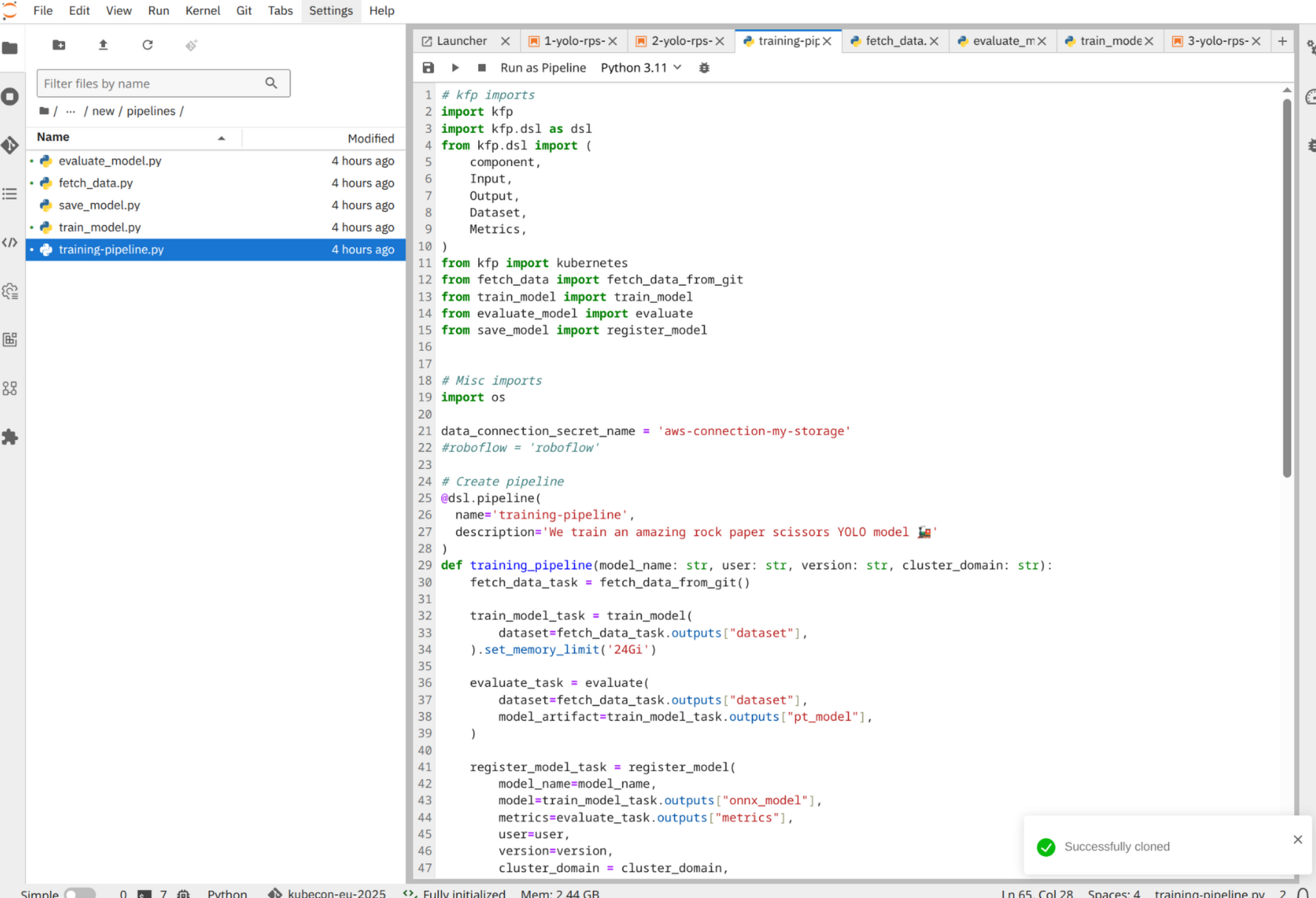
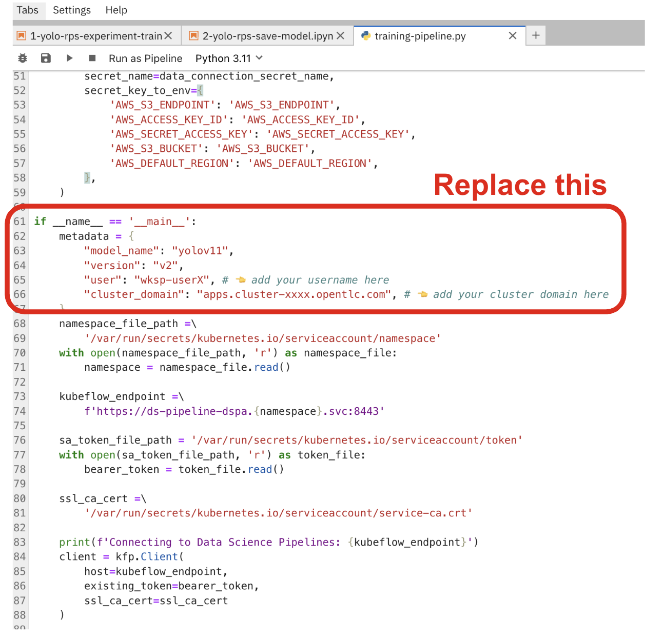
Scroll down in the code and replace the following code with your username and cluster domain:
if __name__ == '__main__':
    metadata = {
        "model_name": "yolov11",
        "version": "v2",
        "user": "{user}",
        "cluster_domain": "{openshift_cluster_ingress_domain}",
    }
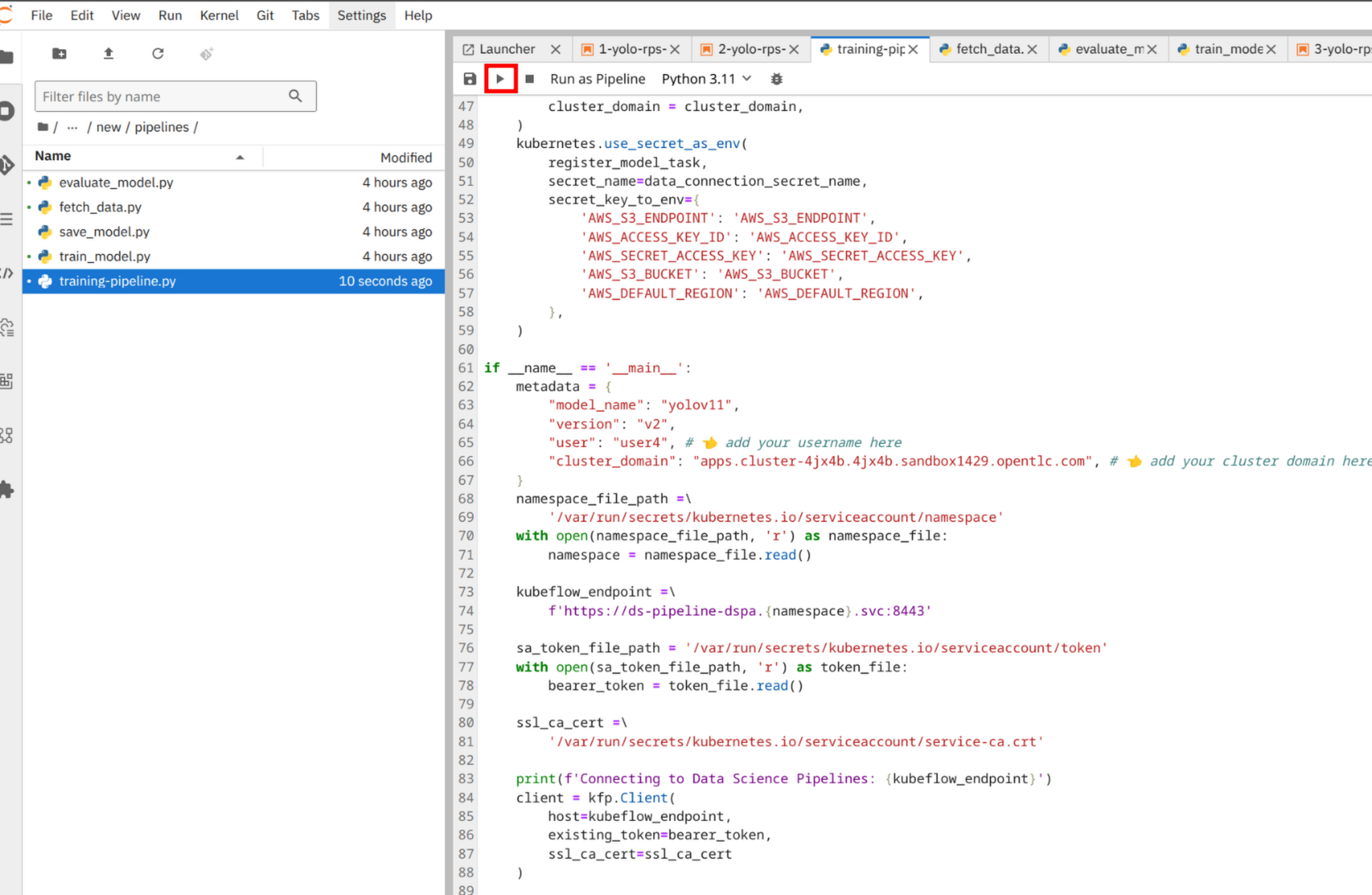
Now go to the top-left of the notebook menu bar and click to the play icon to start the pipeline.
The KFP is now starting on the cluster and you can monitor the progress the dashboard. Go back to the OpenShift AI Dashboard. From the left-side menu, click to Experiments then Experiments and runs. From the list, you should see a kfp-training experiment running.
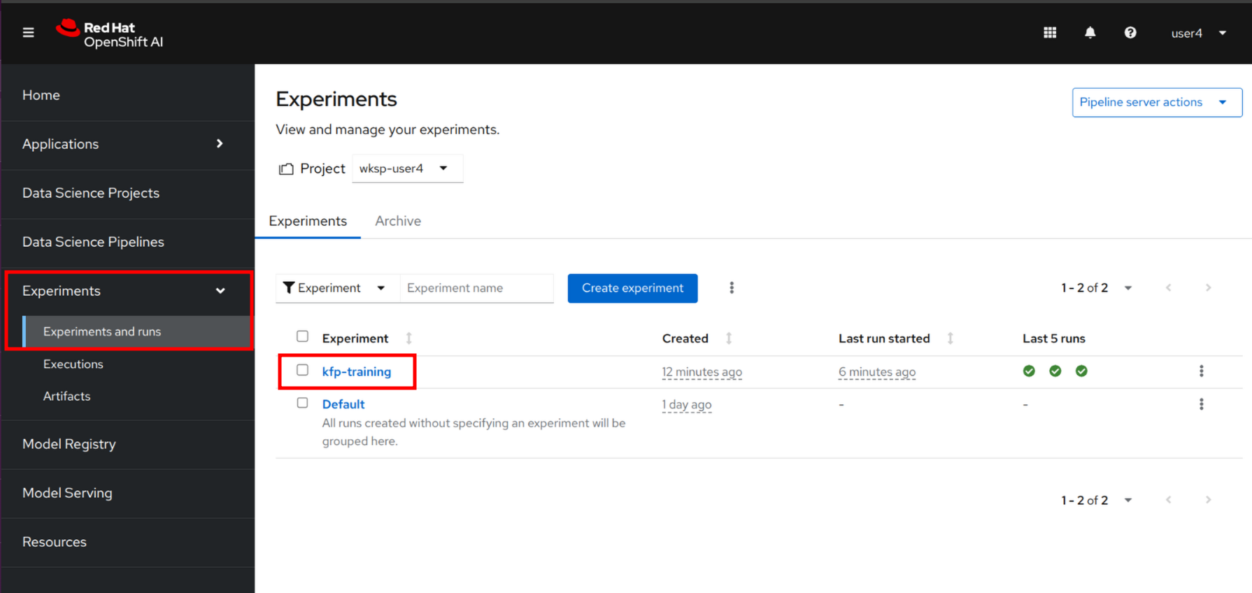
Click to the Kubeflow pipeline to see all details.
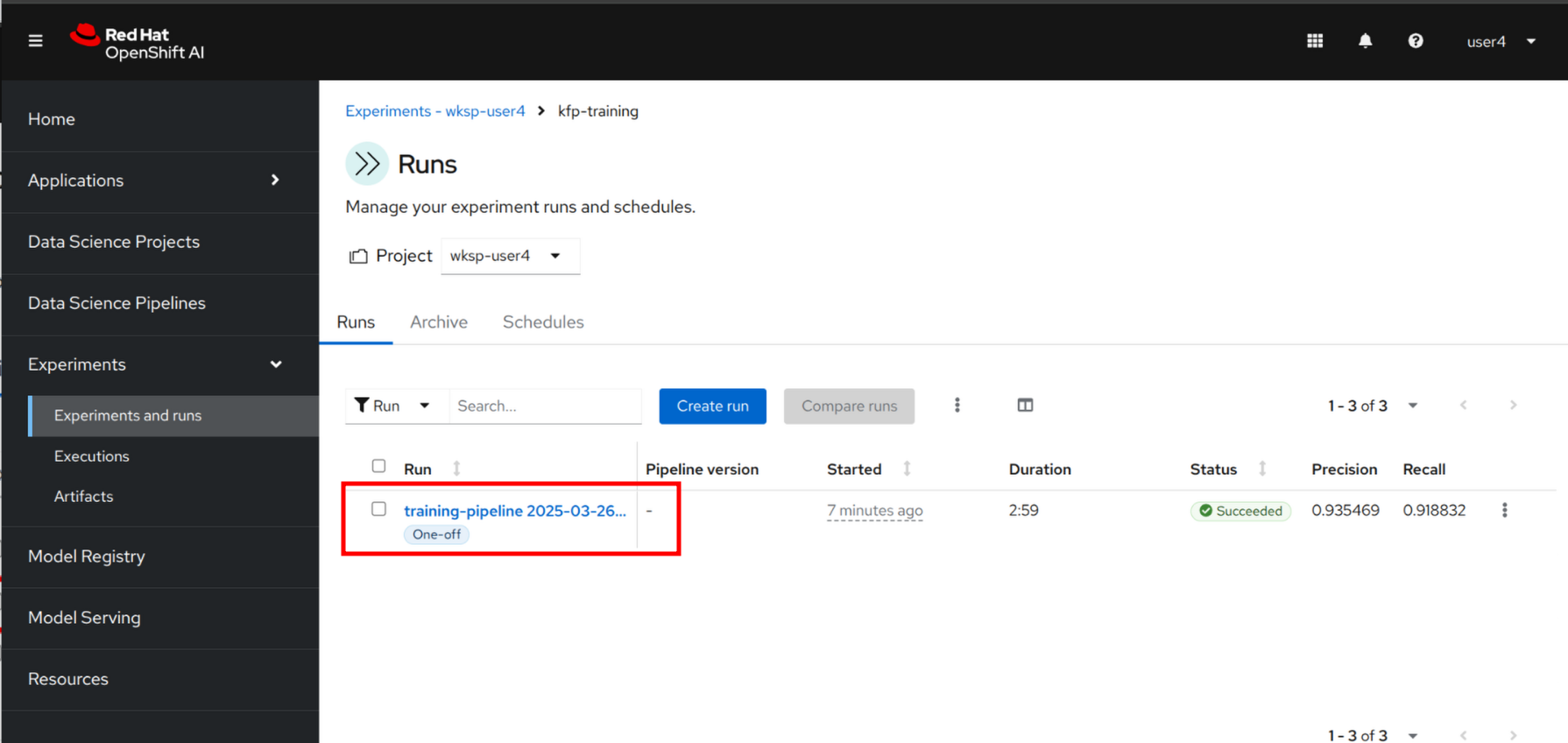
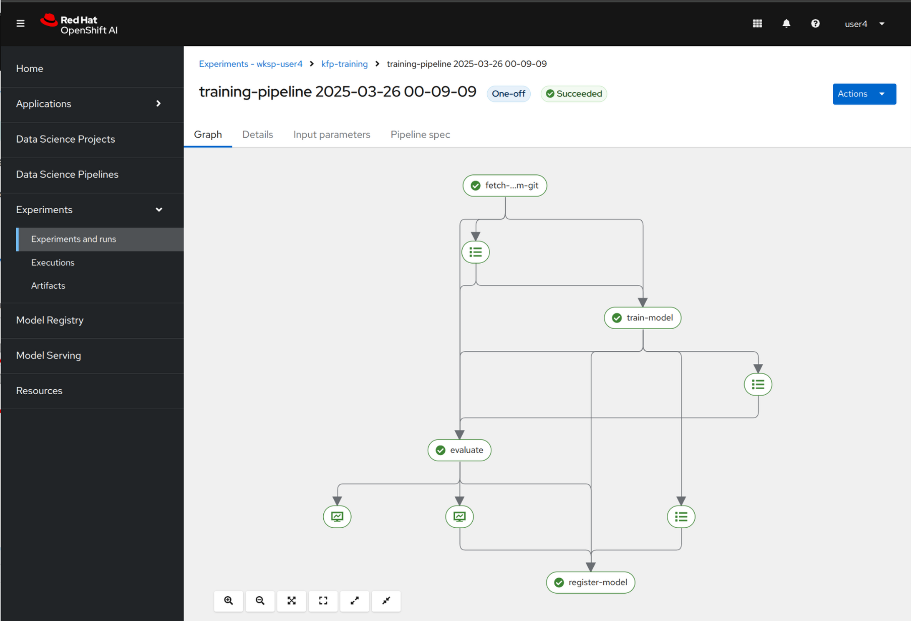
You should see now the graphical representation of the pipeline with all the components involved.
Click to any of them to review status of logs. Note that the pipeline is running for a couple of minutes to finish.
If you click the Evaluate component, you will see the evaluation metrics such as Precision and Recall.
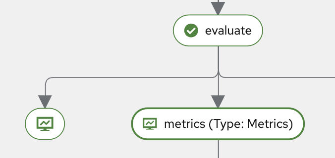
Once you click the Metrics button below Evaluate, navigate to the Visualization tab. There, you’ll find scalar metrics related to model performance after evaluation, such as mAP50, mAP75, mAP, as well as Precision and Recall.
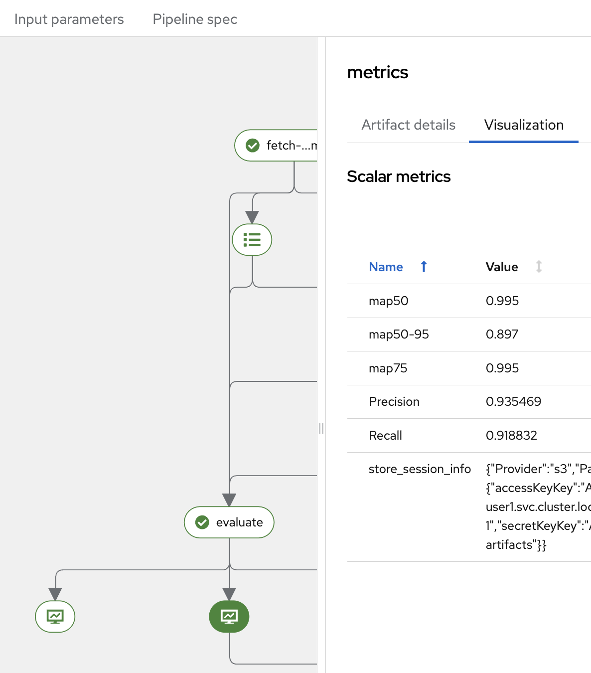
The mAP (mean Average Precision) is a standard metric used in object detection tasks. It summarizes the precision-recall curve into a single value, providing a comprehensive measure of the model’s accuracy across different IoU (Intersection over Union) thresholds.
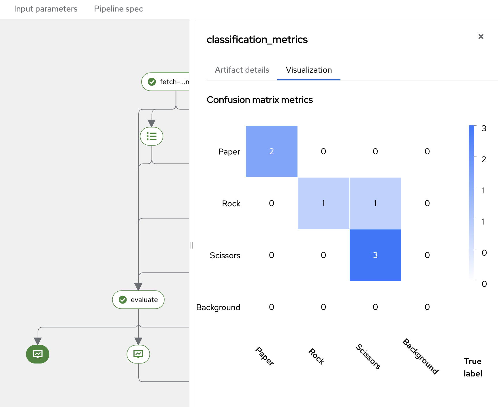
In addition to object detection metrics, you can also review Classification Metrics after the evaluation step.

Click the Classification Metrics button to access these results. You will see the Confusion Matrix, which is a table used to evaluate the performance of a classification model on a test dataset with known target values.
The Confusion Matrix compares the actual target values with the predictions made by the model. It provides insights not only into the number of errors but also the types of errors the classifier makes.
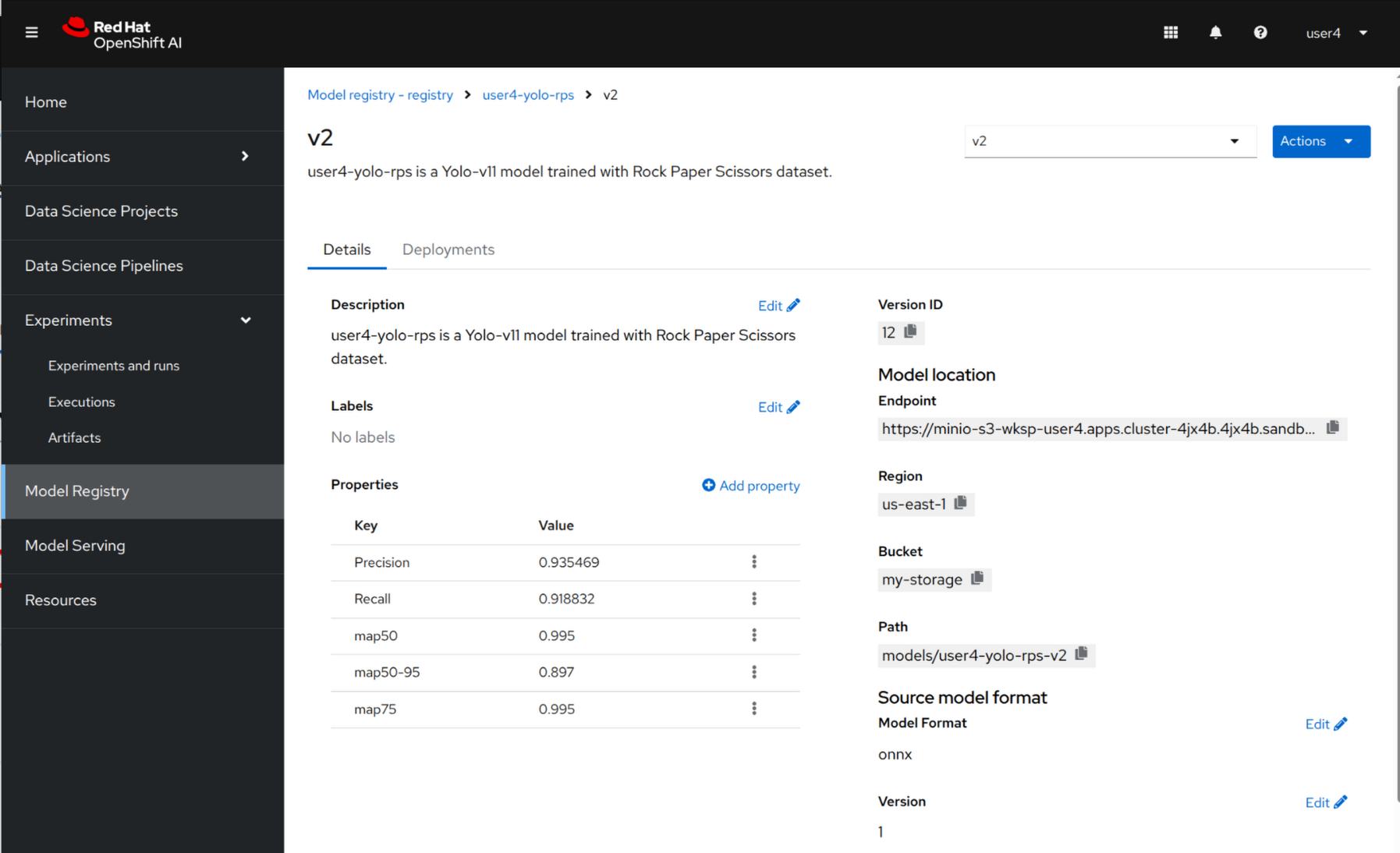
After the Kubeflow pipeline successful run, the new model has been pushed to the Model Registry that you can review.
Navigate to the left-side menu, go to Model Registry and click to the newly created v2.
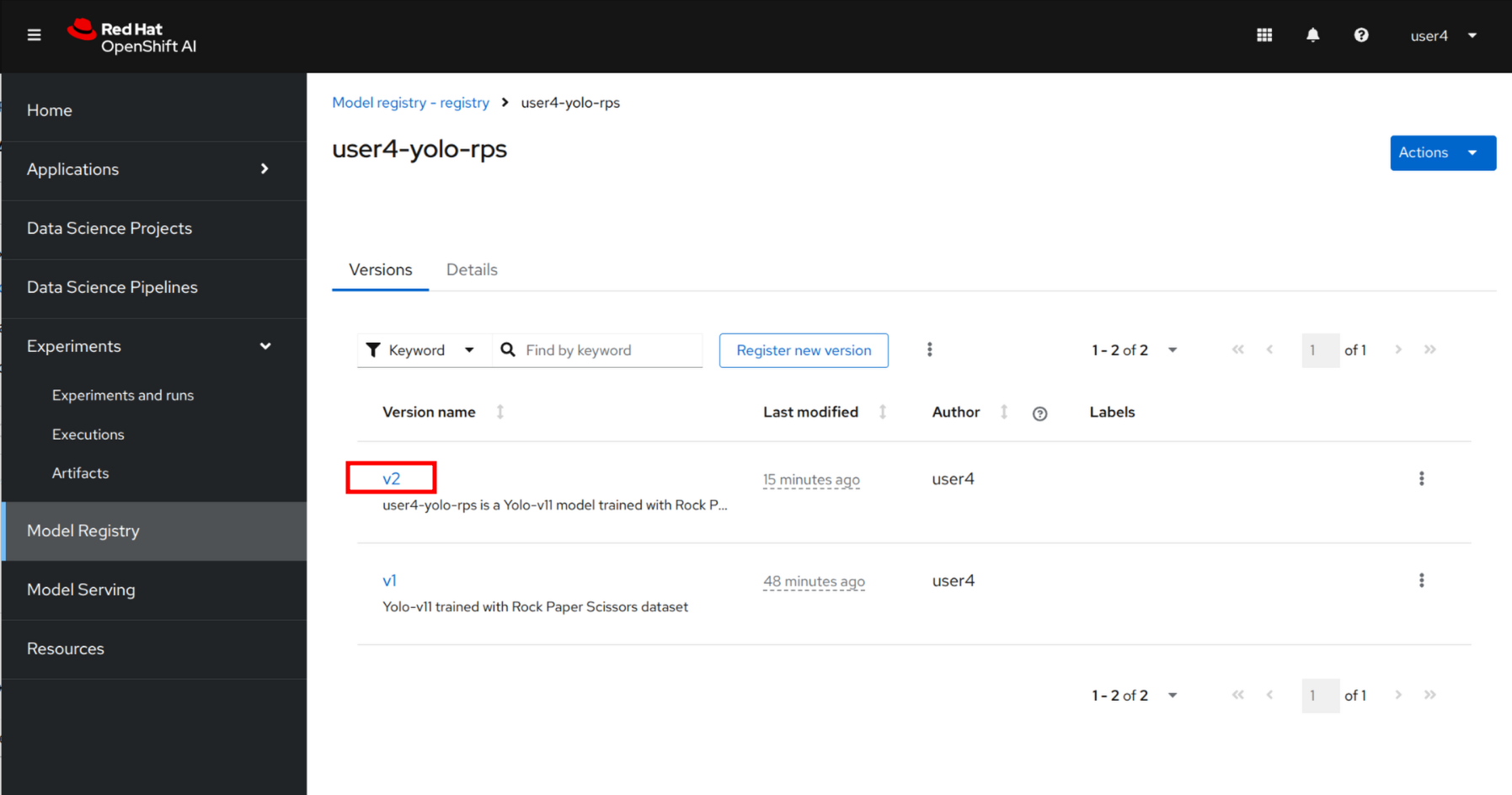
Review all details such as storage location and properties such as Precision and Recall.